Kepler's Equation: Eccentric Anomaly Values at the Quarter-period - Part 2

I am circling back around to post some additional information about elliptical motion at the quarter period.

According to Kepler's Equation for Elliptical Motion,

E = M + e sin(E)                     Equation 1

At the quarter period, the Mean Anomaly, M, becomes π/2 and this equation becomes

E = π/2 + e sin(E)                     Equation 2

A plot of sin(E) at T/4 points for e going from 0 to 1 follows.

This graph, and the data that produced it, are posted on the Desmos website: Plot of sin(E) at the Quarter Period

These data points were computed numerically.
The first column, labelled x₁, contains the e values.
The second column is the Eccentric Anomaly, E, at T/4.
The third column is sin(E) at T/4.
This data is available for use, for anybody interested. Feel free to edit it, or plot functions using the data. However, if you want to save your work, you'll have to create your own account first (it's free.)

Equation 2 can be reduced to

sin(E) = cos[e sin(E)]                     Equation 3

or

x = cos(e x)                     Equation 4

where x = sin(E).

Note that when e = 1, Equation 4 reduces to the familiar form of the definition of the Dottie Number: x = cos(x). In other words, the Dottie Number is just one point on the curve that solves Equation 4.

Now consider the first derivative of E with respect to (w.r.t.) e. Equation 1 is differentiated w.r.t. e to yield

Equation 5 is used to differentiate sin(E) w.r.t. e:

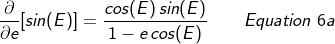
or

A plot of d[sin(E)] / de at the quarter period follows:

This graph, and the data that produced it, are posted on the Desmos website: Plot of d[sin(E)]/de at the Quarter Period

Next, consider the second derivative of sin(E) w.r.t. e:

A plot of d²[sin(E)] / de² at the quarter period follows:

This graph, and the data that produced it, are posted on the Desmos website: Plot of d²[sin(E)]/de² at the Quarter Period

This plot takes a zero value at approximately x = 0.643638135454661. This means the plot for sin(E) values at the quarter period has a point of inflection. For 0 < e < 0.643638135454661 the plot for sin(E) is concave down. For 0.643638135454661 < e < 1 the plot for sin(E) is concave up.

At this point, d[sin(E)] / de = -0.33323545 and
d[cos(E)] / de = -0.5446936

Going through similar steps for cos(E), analogous to Equation 3, values for E_T/4 can be found as the solution to the equation

cos(E) = -sin[e sin(E)]

When e = 1, cos(E_T/4) = - sin(D), where D is the Dottie Number.

Here is a plot of cos(E) at T/4 points for e going from 0 to 1.

The first and second derivatives are

Plots of these derivatives are posted at the following URLs:

First Derivative of cos(E) w.r.t. e at the Quarter Period

Second Derivative of cos(E) w.r.t. e at the Quarter Period

Since the second derivative does not take a zero value over the range of interest ([0, 1]), the curve for cos(E) does not have a point of inflection over this range. Because the concavity of this curve does not change, perhaps it would be more effective to examine features of the cosine curve instead of the sine curve (e.g., a straight line bounding function would not have the risk of the function diverging away from it.)

Here is a plot of cos(E_T/4) with two simple bounding functions:

cos(E) at the Quarter Period with Two Simple Bounding Functions

Investigating the cos(E) curve, recall the equation stated above:

cos(E) = -sin[e sin(E)]

Also, consider the infinite series definition of the sine function:

In the present case, x = e sin(E). Notice that a factor of e is present in all terms.

So, cos(E) can be stated in the form

cos(E) = -e F(e)

where F(e) is some function to be determined.

The corresponding form of sin(E) is

sin(E) = √[1 - e² (F(e))²]

What does a plot of F(e) look like? Here is a plot of F(e) = -cos(E)/e:

Graph of -cos(E) divided by e at the Quarter Period

Note that F(e) goes to 1 as e goes to zero,
and it goes to sin(D) as e goes to 1.

In addition, the series representation indicates that the expression at the sin(E) = sin(M) point could be expressed in a similar form:

cos(E_sE=sM) = -sin[(e/2) sin(E)] = - (e/2) F(e/2)

These proposed forms fit the graphs seen so far.

Looking at other properties of E at the quarter period ...
 
 

Kepler’s Equation of Elliptical Motion Solver

Kepler’s Equation of Elliptical Motion is a famous example of an equation for which an exact, analytical, solution is not possible. In its most succinct form, it is stated as follows:

E - e sin(E) = M

where e is the eccentricity of the ellipse described by the motion
(0 < e < 1);
E is the eccentric anomaly; and
M is the mean anomaly, 2 π /T (t is the time since periapse, and T is the period of the motion).
Note that there is no way to express E explicitly (i.e. – E = a simple expression). Solutions are found either (i) by making approximations, or (ii) computing numerical solutions to a desired degree of accuracy. This post considers some aspects of the second option: computing numerical solutions.

The task of computing numerical solutions to Kepler’s Equation of Elliptical Motion (KE) falls into the general category of root-finding. The equation is arranged as follows

E - e sin(E) – M = 0

which is of the general form f(x) = 0.
It is now in the form applicable to the general task of root-finding (i.e. – finding values of x that make the function f(x) equal to 0, called the roots).

The task of root-finding is a well-developed field of mathematics and computer science. As far as I know, all root-finding algorithms take an iterative approach to computing a solution to a desired degree of accuracy: first, an initial guess for the root is made and checked, then a closer solution is approximated and checked, and this process is repeated until the desired accuracy is obtained.

A number of numerical techniques exist for computing solutions to KE. Some are rather simple approaches, such as the bisection method; others are more sophisticated. In fact, the computing power of today’s computers provides the capability for even less-than-optimum techniques to compute solutions in the blink of an eye. However, motivated by a desire to be more pedantic, a few aspects of motion defined by KE can be highlighted, and their influence on the approaches taken to KE’s solution can be observed. First, consider the two figures below, which plot the motion of two variables defined by KE over one period, T. Figure 1 is a graph of E and M versus t; E is the solid red line and M is the dashed blue line. Figure 2 is a graph of sin(E) and sin(M) versus t; sin(E) is the solid red line and sin(M) is the dashed blue line.

 

 

Three factors come into play for optimizing an approach for solving KE:
1) the size of the interval;
2) the algorithm;
3) the initial guess for a root.

The Size of the Interval

The interval in which a root exists is usually input to a root-finding algorithm. If the interval over which a solution will be sought is small, the computer program has less work to do. The smaller the interval is to begin with, the faster it will be narrowed to an acceptable result.

Rearranging KE, we get

E = M + e sin(E)

Because sin(E) alternates between 1 and -1, the magnitude of the second term on the right side of the equation is restricted to e. In other words, E will never be larger than

E = M + e

and never be smaller than

E = M - e

In fact, in most real-world situations, e is quite small; the eccentricities of the orbits of most of the planets around the Sun are much smaller than 1. For example, the eccentricity of the orbit of Mars, which has a comparatively large eccentricity, is about 0.093. In other words, to compute a point in the orbit of Mars using Kepler’s Equation, the first guess would already be accurate to one decimal point because the interval itself is already less than 0.1. Not much more can be done to reduce the size of the interval for the purpose of hastening a solution of KE.

The Algorithm

Picking an appropriate algorithm is another factor that determines how fast a solution to KE is computed. As can be seen from the graphs above, the motion is smooth and there are no irregularities; first--and higher-order--derivatives exist and are continuous. This characteristic makes algorithms that use these derivatives applicable to the task of solving
KE--qualifying it for a wide range of fast-converging root-finding algorithms. The Newton-Raphson method, which uses the function and its first derivative, is often used for this purpose. However, care must be taken to ensure the algorithm does not diverge away from the solution; otherwise, it converges to a solution at a quadratic rate. Furthermore, other algorithms offer quick convergence, for example, Halley's Method converges at a cubic rate and yet other algorithms converge at a quartic rate. These faster-converging algorithms offer these capabilities by including higher-order terms of the Taylor series when forming the approximation for successive iterations.

(Note that the utility to which the title of this post links uses a combination of the bisection and secant method instead of one of these more sophisticated methods. When the utility was first posted, I planned to write other utilities and wanted an algorithm general enough to use for other root-finding problems; not one that was particularly well-suited to a specific problem.)

The Initial Guess for a Solution

The initial estimate for a root could be anywhere within the interval; however, the closer the first guess is to the actual root, the fewer iterations the algorithm has to make to find the actual root (i.e. - the quicker the program will execute).
Consider the first half of the period:     0 < t < T/2.
For this portion of the motion, sin(E) > 0 and M <= E <= M + e. So the initial estimate for E, E_o, should be in this interval.

One often-recommended initial value for E_o is the following:

Another approach for picking E_o would be to compute some points of E and save them in a table. An interpolating function could then be created and used to provide E_o values for future computations of E. This approach would be especially applicable if E values for a particular ellipse, or over a certain range only, were to be computed.

Other schemes for picking for E_o exist, but many of them get more complicated than I would like to examine in this post.

To summarize, consideration of the characteristics of motion defined by KE yields approaches for its solution that are much more efficient than a simple approach that, on the contrary, takes no account of KE’s characteristics. By (i) minimizing the initial size of the interval over which a solution is to be sought, (ii) applying an appropriate algorithm, and (iii) making an excellent initial estimation for a root, solutions can be computed extremely fast. A variety of methods--the simple Bisection Method, the Newton-Raphson Method, Halley’s Method, and even faster converging iterative approaches--are available to suit a user’s needs, or simply to satisfy a desire to be more pedantic. In conclusion, although an exact solution of Kepler’s Equation does not yet exist, many powerful tools and technique are available that allow numerical solutions to be computed quickly and accurately.

This post presented a brief overview of existing information on the topic of solving KE. For the sake of intellectual curiosity, I do enjoy exploring KE; any work that could be considered research-ish (i.e. – any work done toward the goal of discovering new information) will be posted on my other blog: RocketScientists.ca.

Edit: 20 October 2012
My WordPress blog on rocketscientists.ca was hacked so I deleted the entire site, had my host reset the account, and started over. The main site is back up, but I do not know when--or if--the blog side of the site will ever be re-posted, so I will copy some of those posts over to this blog. And the hotlink given in the paragraph above has been edited to point to the home page.