
Discrete Fourier Transform
The Discrete Fourier Transform (DFT) transforms a data sequence--representing motion that presumably includes periodic components, and sampled at uniform intervals--into a sequence of cyclical functions. Specifically, given a sequence of samples, g0, g1, g2, g3, . . . gN - 1, taken at uniform time intervals, t0, t1, t2, t3, . . . tN - 1, the DFT computes coefficients a0, a1, a2, a3, . . . a[N/2] and b1, b2, b3, . . . b[N/2] that best satisfy the following equation:

where the upper limit [N/2] refers to the largest integer in N:
if N is even, [N/2] refers to N/2;
if N is odd, [N/2] refers to (N - 1)/2.
Note that the a-coefficients include an a0 term; the b-coefficients do not. The a0 term is simply the average value of the data points, and is called the DC component:

The balance of the coefficients are computed by taking one of two paths, depending upon whether N is odd or even:
i) N is odd. The next two equations apply for 1 ≤ k ≤ [N/2]:


ii) N is even. The preceding two equations apply for 1 ≤ k < N/2. The coefficients for k = N/2 are not included.
Instead,

and
When N is even, the value for aN/2 is computed via a simpler expression and the computation for bN/2 is eliminated altogether, being replaced by a simple assignment.
The Sample Data
The sample data used on the akiti.ca web page comes from elliptical motion: eccentricity, e = 0.7861513777574233 and T = 1. Elliptical motion is a fundamental motion of nature, it is periodic, and it is sine-like, so it should serve as an informative example. The motion is divided into a specified number of intervals, and the sample data represents values of sin(E) at the interval endpoints.
Note from the example that the a0 term is zero, as expected--elliptical motion does not have a DC component.
Consider another data sequence. Again, sin(E) values over one complete period are used, but this time the motion is divided into twenty intervals, giving twenty-one data points (i.e., N = 21.)
The sin(E) values:
Some notes:
i) The two endpoints are 0, as they should be:
sin(E) = 0 at t = 0 and t = T.
ii) sin(E) = 0 at the mid-point (t = T/2), as it should be.
iii) t5 is T/4 (T/20 * 5 = T/4), so the sixth value in this data set represents sin(ET/4).
Performing a DFT on this sequence yields the following results:
This time, since N is odd, b[N/2] is non-zero.
Complex Variable Form
The results of Fourier Transforms are often stated in complex variable form: z = u + i v, where i indicates the imaginary component. This format can be derived if the original transform definition is expressed in complex format:

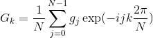
The Gk are computed as
The G, a, and b values are related as follows:
G0 = a0.
Gk = (ak - i bk)/ 2 for 1 ≤ k ≤ [N/2] except if N is even, in which case,
GN/2 = aN/2.
For [N/2] < k < N, the Gk are complex conjugates of the first half.
Using data from the example above:
Comparing Results Between Various Programs
Different programs scale the Fourier coefficients differently, so results will differ. For example, Mathcad and Mathematica use a definition of the transform such that the coefficients are computed as follows:

Note that the ck coefficients are scaled by a factor of 1/√ N instead of 1/N, so the ak and bk values must be multiplied by a factor of √ N to make the numerical values of the coefficients the same. Furthermore, the definition of the ck coefficients does not include a negative factor in the exponential; multiplying the bk coefficients by -1 corroborates the ck values output by Mathcad for 0 ≤ [N/2] (and the balance are the complex conjugates):
In fact, the bk coefficients do not have to be multiplied by -1 to yield a valid result; either the first set of coefficients or their complex conjugates are valid results, so the Gk values for 0 < k < [N/2] can just as well be compared to the ck values for [N/2] < k < N in the first place (and eliminate the need to multiply by -1.)
In this example, the two definitions of the transform are known; the differences in scaling can be taken into account, and the results are seen to verify each other. However, the definition of the transform used internally by some programs may not be known, so it may not be straightforward to corroborate results among different programs. In such cases, the coefficient values must be plugged back into the original definition of the transform to confirm that the original data points are returned. In fact, this is the only way to truly put your mind at ease that a program works. (Always a good idea in any case.)

for j = 0, 1, 2, 3, ... N - 1
where the upper limit [N/2] refers to the largest integer in N:
if N is even, [N/2] refers to N/2;
if N is odd, [N/2] refers to (N - 1)/2.
Note that the a-coefficients include an a0 term; the b-coefficients do not. The a0 term is simply the average value of the data points, and is called the DC component:

The balance of the coefficients are computed by taking one of two paths, depending upon whether N is odd or even:
i) N is odd. The next two equations apply for 1 ≤ k ≤ [N/2]:


ii) N is even. The preceding two equations apply for 1 ≤ k < N/2. The coefficients for k = N/2 are not included.
Instead,

and
bN/2 = 0
When N is even, the value for aN/2 is computed via a simpler expression and the computation for bN/2 is eliminated altogether, being replaced by a simple assignment.
The Sample Data
The sample data used on the akiti.ca web page comes from elliptical motion: eccentricity, e = 0.7861513777574233 and T = 1. Elliptical motion is a fundamental motion of nature, it is periodic, and it is sine-like, so it should serve as an informative example. The motion is divided into a specified number of intervals, and the sample data represents values of sin(E) at the interval endpoints.
Note from the example that the a0 term is zero, as expected--elliptical motion does not have a DC component.
Consider another data sequence. Again, sin(E) values over one complete period are used, but this time the motion is divided into twenty intervals, giving twenty-one data points (i.e., N = 21.)
The sin(E) values:
0
0.817269695391509
0.986037450748215
0.988903757460498
0.918078911674818
0.805917329559989
0.667985913253395
0.513259356200768
0.34762268970459
0.175375726392183
0
-0.175375726392183
-0.347622689704591
-0.513259356200768
-0.667985913253395
-0.805917329559989
-0.918078911674817
-0.988903757460498
-0.986037450748215
-0.817269695391509
0
Some notes:
i) The two endpoints are 0, as they should be:
sin(E) = 0 at t = 0 and t = T.
ii) sin(E) = 0 at the mid-point (t = T/2), as it should be.
iii) t5 is T/4 (T/20 * 5 = T/4), so the sixth value in this data set represents sin(ET/4).
Performing a DFT on this sequence yields the following results:
The ak values follow:
a0 = 0
0.137715757665909
0.0774652995660697
0.0390981194174445
0.0103228847004814
-0.0123006115818896
-0.0301489143722025
-0.0439017247009599
-0.053947159831484
-0.0605247240627844
-0.063778926800584
The bk values follow:
0.913684352303341
0.251136333078314
0.081188081536064
0.0151408910090107
-0.0132569064357189
-0.0240429569155258
-0.0253466725739878
-0.0211727000178036
-0.0138143733065952
-0.00477956981523944
This time, since N is odd, b[N/2] is non-zero.
Complex Variable Form
The results of Fourier Transforms are often stated in complex variable form: z = u + i v, where i indicates the imaginary component. This format can be derived if the original transform definition is expressed in complex format:

for j = 0, 1, 2, 3, ... N - 1.
The Gk are computed as

for k = 0, 1, 2, 3, ... N - 1.
The G, a, and b values are related as follows:
G0 = a0.
Gk = (ak - i bk)/ 2 for 1 ≤ k ≤ [N/2] except if N is even, in which case,
GN/2 = aN/2.
For [N/2] < k < N, the Gk are complex conjugates of the first half.
Using data from the example above:
G0 = 0
0.0688578788329544 - 0.45684217615167i
0.0387326497830349 - 0.125568166539157i
0.0195490597087223 - 0.040594040768032i
0.00516144235024068 - 0.00757044550450537i
-0.00615030579094482 + 0.00662845321785944i
-0.0150744571861012 + 0.0120214784577629i
-0.0219508623504799 + 0.0126733362869939i
-0.026973579915742 + 0.0105863500089018i
-0.0302623620313922 + 0.00690718665329759i
-0.031889463400292 + 0.00238978490761972i
-0.031889463400292 - 0.00238978490761972i
-0.0302623620313922 - 0.00690718665329759i
-0.026973579915742 - 0.0105863500089018i
-0.0219508623504799 - 0.0126733362869939i
-0.0150744571861012 - 0.0120214784577629i
-0.00615030579094482 - 0.00662845321785944i
0.00516144235024068 + 0.00757044550450537i
0.0195490597087223 + 0.040594040768032i
0.0387326497830349 + 0.125568166539157i
0.0688578788329544 + 0.45684217615167i
Comparing Results Between Various Programs
Different programs scale the Fourier coefficients differently, so results will differ. For example, Mathcad and Mathematica use a definition of the transform such that the coefficients are computed as follows:

for k = 0, 1, 2, 3, ... N - 1.
Note that the ck coefficients are scaled by a factor of 1/√ N instead of 1/N, so the ak and bk values must be multiplied by a factor of √ N to make the numerical values of the coefficients the same. Furthermore, the definition of the ck coefficients does not include a negative factor in the exponential; multiplying the bk coefficients by -1 corroborates the ck values output by Mathcad for 0 ≤ [N/2] (and the balance are the complex conjugates):
0
0.3155464419461 + 2.0935138528634i
0.177495299497 + 0.5754256280425i
0.0895850458804 + 0.1860252645836i
0.0236527002651 + 0.0346921395689i
-0.0281842418341 - 0.0303753886113i
-0.0690798411157 - 0.055089334998i
-0.1005914882906 - 0.0580765228428i
-0.1236084717278 - 0.0485127502491i
-0.138679564717 - 0.0316527056779i
-0.1461358799034 - 0.0109513702338i
-0.1461358799034 + 0.0109513702338i
-0.138679564717 + 0.0316527056779i
-0.1236084717278 + 0.0485127502491i
-0.1005914882906 + 0.0580765228428i
-0.0690798411157 + 0.055089334998i
-0.0281842418341 + 0.0303753886113i
0.0236527002651 - 0.0346921395689i
0.0895850458804 - 0.1860252645836i
0.177495299497 - 0.5754256280425i
0.3155464419461 - 2.0935138528634i
In fact, the bk coefficients do not have to be multiplied by -1 to yield a valid result; either the first set of coefficients or their complex conjugates are valid results, so the Gk values for 0 < k < [N/2] can just as well be compared to the ck values for [N/2] < k < N in the first place (and eliminate the need to multiply by -1.)
In this example, the two definitions of the transform are known; the differences in scaling can be taken into account, and the results are seen to verify each other. However, the definition of the transform used internally by some programs may not be known, so it may not be straightforward to corroborate results among different programs. In such cases, the coefficient values must be plugged back into the original definition of the transform to confirm that the original data points are returned. In fact, this is the only way to truly put your mind at ease that a program works. (Always a good idea in any case.)
Labels: calculator, DFT, FFT, fourier, fourier analysis, fourier transform, math, mathematics
posted by David_B | 5:34 PM
![]()
0 Comments:
Post a Comment
<< Home